MLOps Pipelines: From Training to Production Without the Breakage
A technical guide to building a robust MLOps pipeline — covering data versioning, experiment tracking, CI/CD for models, deployment patterns, and drift monitoring.
By Institute for Joint Cognition & AI · 12 min · 20 February 2025
Most ML projects fail not because the model is wrong, but because the infrastructure around it is. The model trains cleanly in a notebook, scores well on a held-out test set, and then something breaks between that local run and the moment a request hits the production endpoint. Sometimes it breaks loudly. More often it breaks silently — predictions degrade over weeks while dashboards show the service is “up.”
The discipline that tries to prevent this is MLOps: the set of practices, tools, and architectural patterns that connect model development to reliable production systems. It borrows from DevOps and data engineering, but it has its own failure modes that neither field fully anticipated.
This article walks through the full pipeline, from raw data to a monitored deployment, with attention to the specific places where things actually go wrong.
What Does an End-to-End MLOps Pipeline Actually Include?
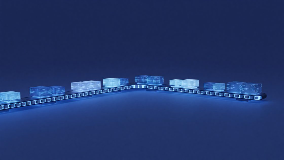
A mature MLOps pipeline is not a single tool. It is a chain of systems, each responsible for a stage of the model lifecycle:
- Data versioning and ingestion — capturing raw data with immutable snapshots and lineage records
- Feature pipelines — transforming raw data into model inputs, consistently, across training and serving
- Experiment tracking — logging hyperparameters, metrics, artifacts, and code versions for every training run
- Model registry — a catalog of trained model artifacts with metadata, stage labels (staging, production, archived), and approval gates
- CI/CD for models — automated testing and promotion pipelines that treat model artifacts the way software pipelines treat binaries
- Deployment — serving infrastructure with rollout strategies (shadow, canary, blue-green)
- Monitoring — detection of data drift, concept drift, and data-quality degradation in production
- Retraining triggers — automated or semi-automated mechanisms that respond to monitoring signals
Each stage produces artifacts and metadata that the next stage consumes. When that chain breaks — when a feature is computed differently in training than in serving, or when a retrained model is promoted without validation — the failure is often invisible until users notice.
Data Versioning: Why Raw Data Is Not Enough
The temptation is to treat data as a static input. In practice, source tables change schema, upstream pipelines add or drop columns, and the same query executed six months apart returns different rows. Without versioning, a model trained “on the same data” as a previous run may actually be trained on something meaningfully different.
Effective data versioning requires:
- Immutable snapshots — a copy of the exact dataset used for training, stored with a content hash or timestamp, not just a pointer to a live table
- Schema versioning — tracking column names, types, and semantics separately from row content
- Lineage metadata — recording which upstream sources, queries, and transformations produced the snapshot
Tools like DVC, Delta Lake, and Apache Iceberg provide snapshot isolation at different levels of the stack. The right choice depends on data scale and warehouse infrastructure, but the principle is the same: a training run must be able to reproduce its inputs exactly, even months later.
This matters especially for reproducibility. The Hidden Technical Debt in Machine Learning Systems paper (Sculley et al., NeurIPS 2015) identified data dependencies as one of the most dangerous sources of long-term maintenance debt in ML systems — dependencies that accumulate invisibly until they cause a production failure.
Feature Pipelines and Training-Serving Skew
Training-serving skew is the single most common cause of silent production degradation. It occurs when the feature values a model sees during training differ from the feature values it sees when scoring live requests — not because the world changed, but because two separate code paths computed the same feature differently.
Common causes:
- Duplicate transformation logic — training uses a Pandas pipeline, serving uses a SQL query, and they disagree on how to handle nulls or encode categoricals
- Timestamp leakage — training joins on future data that would not be available at inference time
- Aggregation window mismatch — a 30-day rolling average computed over a snapshot during training versus a streaming window during serving
The fix is a single feature pipeline that executes the same transformation code in both contexts. Feature stores (Feast, Tecton, Hopsworks) are one approach — they precompute features and serve them from a shared store, so training and serving read the same values. An alternative is a library-based approach: define transformations as versioned Python functions, import them in both the training job and the inference server, and test that both paths produce identical outputs for identical inputs.
Whichever approach you use, write integration tests that compare training-time and serving-time feature values on the same raw inputs before any model goes to production.
Experiment Tracking: What to Log and Why
Without experiment tracking, model development is archaeology. When a production incident forces you to understand why a model behaves a certain way, you need to be able to reconstruct the exact run that produced it — code version, dataset version, hyperparameters, environment, and metrics.
A minimal experiment tracking setup logs:
- Code version — git commit SHA of the training code
- Data version — hash or identifier of the dataset snapshot
- Hyperparameters — all configurable values, not just the ones you tuned
- Metrics — training loss, validation metrics, and any business-proxy metrics evaluated at training time
- Artifacts — the serialized model, preprocessing objects, and any thresholds or metadata the serving layer will need
- Environment — Python version, library versions, hardware configuration
MLflow, Weights & Biases, and Neptune are widely used. The specific tool matters less than the discipline: every training run that produces a candidate model should be tracked, and the tracking record should be the authoritative source for promotion decisions.
One discipline worth enforcing: experiments should be runnable from a clean environment using only the logged parameters and the referenced data version. If you cannot reproduce a run from its tracking record alone, the tracking record is incomplete.
The Model Registry and CI/CD for Models
In software, a CI/CD pipeline takes source code, runs tests, and promotes a build artifact through environments (dev → staging → production). An MLOps pipeline does the same for model artifacts, but with additional validation steps specific to ML:
- Evaluation against a held-out test set — with a gate on minimum acceptable metrics
- Comparison against the current production model — the challenger must beat or match the champion on agreed metrics before promotion
- Behavioral tests — unit tests for model behavior: known inputs should produce expected output ranges, sensitive inputs should be handled consistently
- Serving infrastructure tests — latency and throughput benchmarks under load, confirming the artifact loads and runs within SLA
The model registry holds trained artifacts with metadata and stage labels. Promotion is explicit: a model moves from “candidate” to “staging” to “production” only when it passes the gate for that transition. Rollback is equally explicit: if a production model fails a monitoring check, the registry enables immediate reversion to the previous artifact.
This is also the point where compliance requirements intersect. If your domain requires audit trails (finance, healthcare, regulatory contexts), the registry’s promotion history — with timestamps, approver identities, and test results — is the artifact that satisfies those requirements.
Deployment Patterns: Shadow, Canary, and Blue-Green
Promoting a model to production does not have to mean replacing the current model immediately. Three deployment patterns reduce risk:
Shadow deployment runs the new model in parallel with the current model. Production traffic is served by the current model; the new model receives copies of the same requests and logs its outputs, but those outputs are never returned to users. Shadow mode is the lowest-risk way to validate that a model behaves sensibly on real traffic before it affects anyone.
Canary deployment routes a small percentage of live traffic (1–5%) to the new model while the remainder goes to the current model. Unlike shadow mode, canary predictions are real — users in the canary group receive them. This is appropriate when shadow data is insufficient and you need to measure business metrics (conversion, engagement) rather than just model metrics.
Blue-green deployment maintains two identical serving environments. The “blue” environment serves all production traffic; the “green” environment runs the new model. A switch (load balancer or DNS) flips traffic from blue to green atomically. Rollback is equally atomic — flip the switch back. Blue-green is well suited to batch inference or to cases where gradual rollout is not needed.
For latency-sensitive applications, it is worth reading how organizations approach model inference cost optimization before committing to a serving architecture — deployment patterns interact tightly with serving infrastructure choices. The same pipeline discipline applies regardless of model type; teams shipping computer-vision systems can see how these deployment and latency concerns play out concretely in image segmentation in production.
Monitoring: Drift, Data Quality, and What Actually Breaks
A deployed model does not stay accurate indefinitely. The world changes, upstream data pipelines change, and user behavior changes. Monitoring detects these changes before they cause noticeable harm.
Data drift is a change in the statistical distribution of model inputs. If a model was trained on data where a feature had a mean of 45 and a standard deviation of 12, and the production distribution shifts to a mean of 60, the model may still produce outputs — but those outputs are extrapolations from an out-of-distribution input. Population Stability Index (PSI) and Kolmogorov-Smirnov tests are common statistical tools for detecting input drift.
Concept drift is a change in the relationship between inputs and the correct output. The input distribution may be stable, but the world has changed in a way that makes the model’s learned mapping wrong. Concept drift is harder to detect because it requires ground truth labels — knowing what the correct output was for past predictions.
Data quality degradation includes null rates, out-of-range values, type mismatches, and schema changes in upstream data. These often indicate upstream pipeline problems rather than model problems, but they affect model behavior immediately and can be detected without labels. Monitoring data quality at the feature pipeline boundary — before data reaches the model — catches these failures earlier than monitoring model outputs.
Prediction distribution shift — monitoring the distribution of model outputs over time — provides a label-free signal that something may have changed, even when ground truth is unavailable. A sudden spike in high-confidence predictions, or a collapse in the distribution toward a single class, is often detectable before users report problems.
Effective monitoring requires baselines: reference distributions captured from the training dataset or an early production window, against which current distributions are compared. Without baselines, anomaly detection has no anchor.
For systems that incorporate retrieval alongside model inference, the same monitoring principles apply to the retrieval layer — a topic covered in more depth in retrieval-augmented generation in practice.
Retraining Triggers and Reproducibility
Retraining is not free. It requires compute, engineering time, and validation. Triggering it too eagerly wastes resources; triggering it too late allows a degraded model to affect users. The right approach is explicit triggers with defined thresholds:
- Scheduled retraining — a baseline cadence (weekly, monthly) that ensures the model sees recent data regardless of detected drift
- Metric-based triggers — retraining fires when a monitored metric crosses a threshold (PSI > 0.2 on a key feature, accuracy below a floor on a labeled evaluation set)
- Event-based triggers — retraining fires when a known upstream event occurs (a product launch, a regulatory change, a data pipeline migration)
Automated retraining requires that the full training pipeline is itself reproducible and automated. A retrained model should go through the same CI/CD gates as any other candidate — it is not automatically better than the current production model just because it is newer.
Reproducibility deserves emphasis. A reproducible training run is one where, given the same data version and hyperparameters, you can recover the same model artifact (or a statistically equivalent one, for stochastic training). This requires controlling random seeds, pinning library versions, and using deterministic data loading. It also requires that experiment tracking captures enough to reconstruct the run — not just the hyperparameters, but the exact training code and environment.
Reproducibility is not just a debugging convenience. It is the mechanism by which you can investigate a production incident, understand what the model learned, and make a principled decision about whether to retrain or roll back.
Frequently Asked Questions
What is training-serving skew?
Training-serving skew occurs when the features a model receives during training differ from the features it receives during inference — not because the world changed, but because two separate code paths compute the same transformation differently. It is one of the most common causes of silent production degradation and is prevented by sharing a single transformation implementation across both contexts.
How is CI/CD for machine learning models different from software CI/CD?
Software CI/CD validates that code compiles, passes unit tests, and behaves correctly. ML CI/CD must additionally validate that a trained artifact meets performance thresholds, outperforms the current production model on agreed metrics, and behaves correctly on behavioral test cases. The artifact being promoted is a binary model file, not source code, so the pipeline must also verify that the artifact loads and runs correctly in the target serving environment.
What is model drift and how do I detect it?
Model drift is a general term for the degradation of model accuracy over time. It has two main causes: data drift (the distribution of inputs changes) and concept drift (the relationship between inputs and correct outputs changes). Data drift is detectable using statistical tests on feature distributions, compared against a reference baseline. Concept drift requires ground truth labels and is typically measured by evaluating model predictions against delayed ground truth on a rolling window.
When should a model be retrained?
A model should be retrained on a defined schedule (to incorporate recent data), when a monitored drift metric crosses a defined threshold, or when a known upstream event makes the training data unrepresentative of current conditions. Retraining should not be automatic promotion — a retrained model is a candidate that must pass the same validation gates as any other candidate before replacing the production model.
What is a model registry and why does it matter?
A model registry is a versioned catalog of trained model artifacts, each tagged with metadata — training run ID, data version, evaluation metrics, and stage (candidate, staging, production, archived). It provides a single source of truth for what is deployed and why, enables rollback to a previous artifact, and creates the audit trail required in regulated domains. Without a registry, promotion and rollback are manual and error-prone.